Introduction
We begin by first reviewing Kirsch's solution for the basic case of uniaxial tension, and then use superposition techniques to develop solutions for the more complex cases of equibiaxial tension and shear. This is followed by the solution for general 2-D loading. And the page concludes with stress concentrations in finite width plates.
Uniaxial Tension - Kirsch's Solution (1898)
Kirsch's solution for stresses at a hole are for the case of uniaxial tension in an infinite plate. Uniaxial tension is represented by the remote stress, \(\sigma_\infty\). The hole has radius, \(a\), the radial coordinate is \(r\) (which is meaningless when \(r \lt a\)), and \(\theta = 0\) aligns with the remote loading direction. We will see that the famous factor-of-three stress concentration occurs at \(\theta = \pm\, 90^\circ\).
There is no need to review the derivation. The solution for the stress state around a hole is
\[ \begin{eqnarray} \sigma_{rr} & = & {\sigma_\infty \over 2} \left( 1 - \left( a \over r \right)^2 \right) + {\sigma_\infty \over 2} \left( 1 - 4 \left( a \over r \right)^2 \! \! + 3 \left( a \over r \right)^4 \right) \cos 2\theta \\ \\ \sigma_{\theta \theta} & = & {\sigma_\infty \over 2} \left( 1 + \left( a \over r \right)^2 \right) - {\sigma_\infty \over 2} \left( 1 + 3 \left( a \over r \right)^4 \right) \cos 2\theta \\ \\ \tau_{r \theta} & = & - {\sigma_\infty \over 2} \left( 1 + 2 \left( a \over r \right)^2 \! \! - 3 \left( a \over r \right)^4 \right) \sin 2\theta \end{eqnarray} \]
At Infinity
At \(r = \infty\), all the \(a / r\) terms go to zero, leaving\[ \begin{eqnarray} \sigma_{rr} & = & {\sigma_\infty \over 2} + {\sigma_\infty \over 2} \cos 2\theta \\ \\ \sigma_{\theta \theta} & = & {\sigma_\infty \over 2} - {\sigma_\infty \over 2} \cos 2\theta \\ \\ \tau_{r \theta} & = & - {\sigma_\infty \over 2} \sin 2\theta \end{eqnarray} \]
and \(\sigma_{rr} = \sigma_\infty\) when \(\theta = 0^\circ\) and \(180^\circ\), while \(\sigma_{\theta \theta} = \sigma_\infty\) when \(\theta = \pm \, 90^\circ\), as they must be. The shear stress, \(\tau_{r \theta}\), is simply the result of coordinate transformations on \(\sigma_\infty\).
At The Hole
\[ \begin{eqnarray} \sigma_{rr} & = & 0 \\ \\ \sigma_{\theta \theta} & = & \sigma_\infty ( 1 - 2 \cos 2\theta ) \\ \\ \tau_{r \theta} & = & 0 \end{eqnarray} \]
The radial stress, \(\sigma_{rr}\), and the shear stress, \(\tau_{r \theta}\), are zero at the hole because it is a free surface.
It is the hoop stress, \(\sigma_{\theta \theta}\), that merits attention. At \(\theta = 0\), \(\sigma_{\theta \theta} = - \sigma_\infty\), so the hoop stress is actually compressive. However, it is at \(\theta = \pm \, 90^\circ\) that \(\sigma_{\theta \theta} = 3 \, \sigma_\infty\) and the factor-of-three stress ratio occurs. This ratio is called the Stress Concentration Factor and is discussed below.
This is the largest stress at the hole, and therefore the first value to compare to a material's yield strength to check for yielding. The stress state is uniaxial, so the \(\sigma_{\theta \theta}\) value is also the effective or von Mises stress that can be directly compared to the material's yeild strength.
Note that the stress components at the hole are independent of the size of the hole itself. This is related to the fact that the plate is infinitely large, so the hole's size is inconsequential relative to the plate.
Stress Concentration Factor, \(K_t\)
The Stress Concentration Factor, \(K_t\), is the ratio of maximum stress at a hole, fillet, or notch, (but not a crack) to the remote stress. For our case of a hole in an infinite plate, \(K_t = 3.\)Do not confuse the Stress Concentration Factor here with the Stress Intensity Factor used in crack analyses. The two are completely different. For starters, a Stress Concentration Factor is dimensionless, while a Stress Intensity Factor is not. Stress Intensity Factors will be discussed on later pages.
Keep in mind that everything here applies to an empty hole. Do not confuse this situation with that of a hole containing a fastener. That scenario has infinitely many variations depending on the relative loads carried by the fastener and the plate (with the hole).
Stress State Schematics
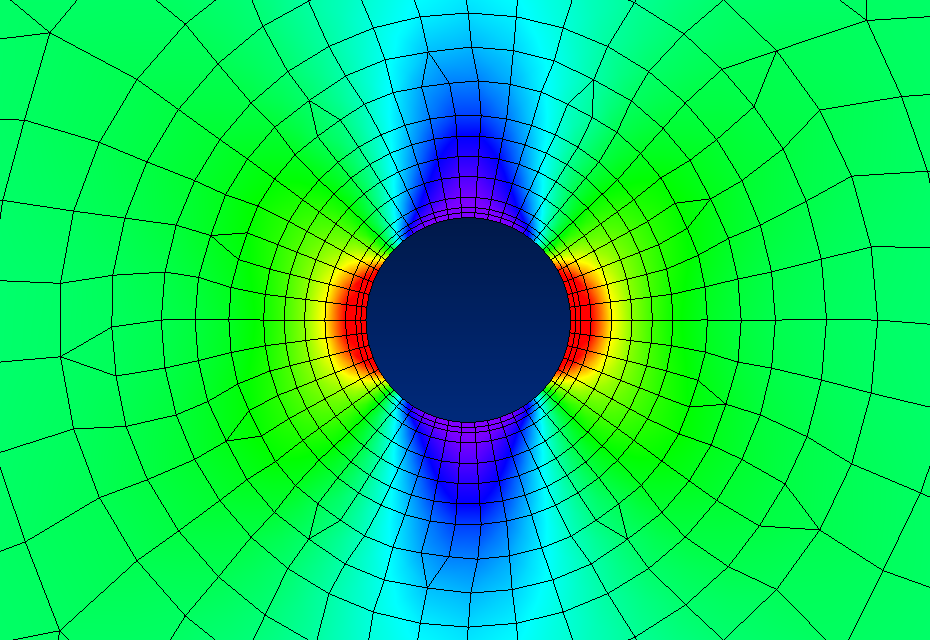
The first sketch here plots the hoop stress, \(\sigma_{\theta \theta}\), at \(\theta = \pm \, 90^\circ\) as a function of \(r\). It shows the factor-of-three concentration at the hole's edge and how it quickly dissipates away with increasing \(r\). The stress concentration is small again at one diameter distance from the hole's edge, and indeed negligible at two diameters distance. In finite element analyses, this steep gradient necessitates a very fine mesh in the radial direction in order to accurately model the stress and strain field.
The complex stress field around a hole is summarized in the sketch below. It shows a series of stress states at the hole edge, one radius away, and one diameter away. The normal stresses are symmetric, left and right, so conditions on either side also apply to the other. This is reflected in the equations by the fact that \(\cos(2\theta) = \cos(-2\theta)\). The shear stresses on one side are negative of the other, and this is reflected by \(\sin(2\theta) = -\sin(-2\theta)\).
There are no shear stresses at \(\theta = 0^\circ, 90^\circ, 180^\circ,\) etc. So the normal stresses are in fact principal stresses as well at these angles.
Note that the stress states at \(\theta = 45^\circ\) and \(\theta = 135^\circ\) are the same. They are indeed identical, meaning they have the same principal stress values. It is only the displays that are different due to the different orientations of the coordinate systems. This is reflected in the orientations of the squares. The set at \(\theta = 45^\circ\) are aligned with the hole, so the coordinate system is polar and the stress components are \(\sigma_{rr}, \sigma_{\theta \theta},\) and \(\tau_{r \theta}\).
The stress states at \(\theta = 135^\circ\) are aligned with the external uniaxial load , \(\sigma_\infty\). So the coordinate system is rectangular and the stress components are \(\sigma_{xx}, \sigma_{yy},\) and \(\sigma_{xy}\).
The sketch below addresses the subject of hole size and its (lack of) influence on the stresses around it. The counter intuitive result is that the factor-of-three stress concentration is independent of hole size. A very small hole produces the same stress concentration as a very large hole (in an infinite plate).
The red curves show, qualitatively, the flow of force around the hole in a manner similar to streamlines in a fluid flow field. The spacing between curves, which is a minimum at the hole's sides, reflects stress concentrations.
Continuing the flow field analogy... the hole's height provides early warning to the force flow field that it must divert around the hole. The flow must divert more for a wider hole, but then a wider hole is also taller, so it alerts the flow earlier. The net result is that the stress concentration at the hole is always three, regardless of the hole's size.
This is relevant because of its contrast to ellipses and cracks. Consider that a crack has no height to provide early warning to the hypothetical flow field that it must divert. Nevertheless, the longer the crack, the more the flow must divert, hence the greater the stress concentration. This will be addressed more rigorously in following webpages.
Equibiaxial Loading
\[ \begin{eqnarray} \sigma_{rr} & = & \sigma_\infty \left( 1 - \left( a \over r \right)^2 \right) \\ \\ \sigma_{\theta \theta} & = & \sigma_\infty \left( 1 + \left( a \over r \right)^2 \right) \\ \\ \tau_{r \theta} & = & 0 \end{eqnarray} \]
Shear Loading
The effects of shear loading can be determined by superposition of its principal stresses. The figure below shows the two principal stresses oriented at ± 45°, The first one is positive and numerically equal to the shear stress value. The second one is negative. The result is that shear loading leads to a factor of four stress concentration at the hole.
General 2-D Loading
Linear superposition can be used to obtain analytical solutions for the stress field under general 2-D loading conditions. In this case, \(\sigma_\infty\) is replaced by \(\sigma_{xx}\), then \(\sigma_{yy}\), and finally positive and negative principal stresses equal to the shear stress, \(\tau_{xy}\).
\(\theta = 0^\circ\) initially corresponds to \(\sigma_{xx}\). Then \(\theta + 90^\circ\) is substituted for \(\theta\) when \(\sigma_\infty = \sigma_{yy}\). And \(\theta \pm 45^\circ\) is used with the principal stresses for \(\tau_{xy}\).
The resulting equations are...
\[ \begin{eqnarray} \sigma_{rr} & = & {\sigma_{xx} + \sigma_{yy} \over 2} \left( 1 - \left( a \over r \right)^2 \right) + \left( 1 - 4 \left( a \over r \right)^2 \! \! + 3 \left( a \over r \right)^4 \right) \left( \left( {\sigma_{xx} - \sigma_{yy} \over 2} \right) \cos 2\theta + \tau_{xy} \sin 2\theta \right) \\ \\ \sigma_{\theta \theta} & = & {\sigma_{xx} + \sigma_{yy} \over 2} \left( 1 + \left( a \over r \right)^2 \right) - \left( 1 + 3 \left( a \over r \right)^4 \right) \left( \left( {\sigma_{xx} - \sigma_{yy} \over 2} \right) \cos 2\theta + \tau_{xy} \sin 2\theta \right) \\ \\ \tau_{r \theta} & = & \left( 1 + 2 \left( a \over r \right)^2 \! \! - 3 \left( a \over r \right)^4 \right) \left( \left( {\sigma_{yy} - \sigma_{xx} \over 2} \right) \sin 2\theta + \tau_{xy} \cos 2\theta \right) \\ \end{eqnarray} \]
and the special case of hoop stress at the hole's edge is
\[ \sigma_{\theta \theta} |_{r=a} \; = \left( \sigma_{xx} + \sigma_{yy} \right) - 2 \left( \sigma_{xx} - \sigma_{yy} \right) \cos 2\theta - 4 \, \tau_{xy} \sin 2\theta \]
Finite Width Effects
When working with finite width plates, it is necessary to introduce an additional term, the nominal stress, \(\sigma_\text{nom}\). It is the average stress at the hole due to the reduction in cross section and is related to \(\sigma_\infty\) by
\[ \text{Force} \; = \; \sigma_\infty W \; = \; \sigma_\text{nom} ( W - d ) \]
where \(d\) is hole diameter, \(W\) is plate width, and thickness has been ignored. Solving for \(\sigma_\text{nom}\) gives
\[ \sigma_\text{nom} = { W \over W - d } \; \sigma_\infty \]
The Stress Concentration Factor is then defined as
\[ K_t = {\sigma_\text{max} \over \sigma_\text{nom} } \]
where \(\sigma_\text{max}\) is in this case, the maximum hoop stress, \(\sigma_{\theta \theta}\), at \(\theta = 90^\circ\). Note that the denominator here is NOT \(\sigma_\infty\), but \(\sigma_\text{nom}\) instead. This is standard practice.
The standard graph showing the dependence of \(K_t\) on the dimensionless ratio, \(d / W\), for a plate is shown below. \(d / W = 0\) corresponds to the infinitely wide plate, and indeed, \(K_t = 3\) at this point. The equation for the curve, which is in fact empirical, is
\[ K_t = 3 - 3.14 \left( {d \over W} \right) + 3.667 \left( {d \over W} \right)^2 - 1.527 \left( {d \over W} \right)^3 \]
The graph shows that \(K_t\) decreases toward 2 as \(d / W\) approaches 1, and one might be tempted to conclude that \(\sigma_\text{max}\) therefore decreases as well. But this is absolutely wrong. The reason is that \(K_t\) is no longer the ratio of \(\sigma_\text{max}\) to \(\sigma_\infty\). It is instead the ratio to \(\sigma_\text{nom}\). The ratio to \(\sigma_\infty\) is obtained by
\[ { \sigma_\text{max} \over \sigma_\infty} \; = \; \left( { \sigma_\text{max} \over \sigma_\text{nom} } \right) \! \left( { \sigma_\text{nom} \over \sigma_\infty} \right) \; = \; K_t \, {W \over W - d} \]
And the last term can be manipulated to give
\[ { \sigma_\text{max} \over \sigma_\infty} \; = \; K_t \; {1 \over 1 - \left( d \over W \right) } \]
which permits the entire term to be plotted against the dimensionless parameter, \(d / W\).
Note how the \(\sigma_\text{max} / \sigma_\infty\) curve is initially flat and equal to 3 for all small values of \(d / W\), but then begins to increase dramatically with increasing \(d / W\) at larger values of it. The initial flatness of the curve at small \(d / W\) values can be interpreted as \(\sigma_\text{max}\) initially remaining unchanged as the width, \(W\), is decreased from infinity down to finite values. The initial decrease, relative to infinity, is negligible.
Equally interesting is the fact that the \(\sigma_\text{max} / \sigma_\infty\) ratio never decreases. While the \(K_t\) ratio, relative to \(\sigma_\text{nom}\) always decreases with increasing \(d / W\), the ratio relative to \(\sigma_\infty\) always increases. In other words, increasing the hole diameter or decreasing the plate width in a finite width plate will in fact always increase the maximum stress at the hole.
Can \(\boldsymbol{\sigma_\text{max}}\) exceed \(\boldsymbol{\sigma_\text{yield}}\)?
One last thing to consider... Keep in mind that in reality, no stress can exceed the material's yield strength, \(\sigma_\text{yield}\) (cold-working aside). So how does one resolve a situation in which the computed \(\sigma_\text{max}\) stress is greater than \(\sigma_\text{yield}\)?The resolution is that the computed \(\sigma_\text{max}\) value is incorrect because it is the result of a linear elastic calculation. But in fact, the material will have yielded, rendering the linear elastic solution moot.
References
- Kirsch, E.G., "Die Theorie der Elastizität und die Bedürfnisse der Festigkeitslehre," Zeitschrift des Vereines deutscher Ingenieure, Vol. 42, pp. 797-807, 1898.